Parallelising tasks

As we mentioned in the introduction to this course, an important tool in leveraging modern hardware in the face of stagnating clock speeds is through parallel computation.

Parallel computation is the simultaneous execution of computations across multiple executing units. These maybe cores within a CPU, maybe multiple CPUs (possibly each with multiple cores), and maybe multiple computers systems.

There are a number of distinct types of workload parallelisation that depend on the actual task being executed in parallel and its properties. Let’s look at a few core concepts before examining parallel workflows in R.

Embarassingly parallel problems

In parallel computing, an embarrassingly parallel workload or problem is one where little or no effort is needed to separate the problem into a number of parallel tasks. This is often the case where there is little or no dependency or need for communication between those parallel tasks, or for results between them.

Data parallel problems

One common type of embarassibgy parallel problems are data parallel problems. This is when the same operations is performed on different subsets of same data.

Examples of data parallel problems:

Generating a synthetic person (if their attributes are independent of each other).
Counting the number of occurrences of a given token in individual documents of a corpus.
Analysing many satellite images using the same algorithm for a specific feature.

Map-reduce parallel programming

Many data parallel problem are solved through the map-reduce programming paradigm. The core principles behind ‘map-reduce’ computing approaches involve

splitting the data as input to a large number of independent computations
collecting the results for further analysis

Parallel computing in R

Data parallel map-reduce problems

A good indication that you are dealing with a map reduce problem that could benefit from data parallelisation is if, when profiling, you find that your code is spending a lot of time in function like lapply, Map(), purrr::map and related functions.

All these functions follow a map reduce paradigm where the input is split up into it’s elements, the same function is applied to each element of the input and the results are aggregated together in the end and returned.

In this section, we’ll see how approaches to optimising such computations through parallelisation have evolved in R.

For a thoroughly entertaining introduction to this topic, I highly recommend the following talk by Bryan Lewis at RStudio::conf 2020:

Parallel computing with R using foreach, future, and other packages - RStudio

`parallel` package

The first widely used package for parallelisation was the parallel package which has been shipping along with base R since version 2.14.0. (released in October 2011).

It’s particularly suited to map-reduce data parallel problems as it’s main interface consists of parallel versions of lapply and similar.

Let’s have a look at how we might use parallel package to parallelise a simple computation involving lapply.

First let’s creates a function that lapply will execute called example_fun.

The function takes an integer i as input, sends the process it is running on to sleep for one second and then returns a character string which records the value of i and the process ID that is performing the computation.

example_fun <- function(i) {
    Sys.sleep(1) 
    paste("Running i =", i, "in process:", Sys.getpid())  
}

In our example workflow, we then use lapply to iterate over our data, here a sequence of integers of from 1 to 8. Let’s run our example and time it’s execution

library(tictoc)

data <- 1:8
tic()
lapply(data, example_fun)

[[1]]
[1] "Running i = 1 in process: 4098"

[[2]]
[1] "Running i = 2 in process: 4098"

[[3]]
[1] "Running i = 3 in process: 4098"

[[4]]
[1] "Running i = 4 in process: 4098"

[[5]]
[1] "Running i = 5 in process: 4098"

[[6]]
[1] "Running i = 6 in process: 4098"

[[7]]
[1] "Running i = 7 in process: 4098"

[[8]]
[1] "Running i = 8 in process: 4098"

toc()

8.035 sec elapsed

We can see that lapply iterates through our input vector sequentially, all computation is performed by the same process and execution takes about 8 seconds to run.

`mclapply()`

Now, let’s try and parallelise our computation using the parallel package.

First let’s load it and decide how much compute power on our machine we want to allocate to the task.

library(parallel)

We can do that by first examining how many cores we have available using detectCores()

detectCores()

[1] 10

I’ve got 10 cores available which is the same as the number of my physical cores. Some systems might show more if the system allows hyperthreading. To return the number of physical cores, you can use detectCores(logical = FALSE).

Given I have 10 available, I’ll assign 8 (detectCores() - 2) to a variable n_cores that I can use to specify the number of cores I want to use when registering parallel backends. If you have less cores available, you should assign at least 1 less than what you have available to n_cores.

n_cores <- detectCores() - 2

Tip

A better approach to get the same result more robustly is to use function availableCores(omit = 2L) from the parallely package, especially if core detection is included within package code or will be run on CI. For discussion of this topic, have a look at this blogpost.

Now, on to parallelising our workflow!

One of the simplest functions used early on to parallelise workflows through the parallel packages is mclapply . This can be used as a pretty much drop in replacement for lapply. The main difference is that we use argument mc.cores to specify the number of cores we want to parallelise across.

Let’s create some new data that has length equal to the number of cores we’re going to use and run our computation using mclapply().

data <- 1:n_cores

tic()
mclapply(data, example_fun, mc.cores = n_cores)

[[1]]
[1] "Running i = 1 in process: 4159"

[[2]]
[1] "Running i = 2 in process: 4160"

[[3]]
[1] "Running i = 3 in process: 4161"

[[4]]
[1] "Running i = 4 in process: 4162"

[[5]]
[1] "Running i = 5 in process: 4163"

[[6]]
[1] "Running i = 6 in process: 4164"

[[7]]
[1] "Running i = 7 in process: 4165"

[[8]]
[1] "Running i = 8 in process: 4166"

toc()

1.018 sec elapsed

This worked on my macOS machine!

It and completed in about 1 second and the output shows that each value of i was computed on in a different process. It will also have worked for anyone running the code on a Linux machine.

However! For any Windows users out there, this will not have worked!

That’s because mclapply() uses process forking. One of the benefits of forking is that global variables in the main R session are inherited by the child processes. However, this can cause instabilities and the type of forking used is not supported on Windows machines (and actually can be problematic when running in RStudio too!)

`parLapply()`

If you’d written a package using mclapply() to improve it’s performance but now you wanted to support parallelisation on Windows, you’d have to re-write everything using parLapply() instead.

To use paLapply() we need to create a cluster object to specify the parallel backend using the parallel::makeCluster() function. By default it creates a cluster of type "PSOCK" which uses sockets. A socket is simply a mechanism with which multiple processes or applications running on your computer (or different computers, for that matter) can communicate with each other and will work on any of our local machines. Each thread runs separately without sharing objects or variables, which can only be passed from the parent process explicitly.

We the pass the cluster as the first argument to parLapply() followed by the standard arguments we are used to in lapply.

cl <- makeCluster(n_cores)
cl

socket cluster with 8 nodes on host 'localhost'

tic()
parLapply(cl, data, example_fun)

[[1]]
[1] "Running i = 1 in process: 4168"

[[2]]
[1] "Running i = 2 in process: 4169"

[[3]]
[1] "Running i = 3 in process: 4175"

[[4]]
[1] "Running i = 4 in process: 4173"

[[5]]
[1] "Running i = 5 in process: 4174"

[[6]]
[1] "Running i = 6 in process: 4171"

[[7]]
[1] "Running i = 7 in process: 4170"

[[8]]
[1] "Running i = 8 in process: 4172"

toc()

1.013 sec elapsed

This now works on all systems. It does however includes disadvantages like increased communication overhead (when dealing with larger data), and the fact that global variables have to be identified and explicitly exported to each worker in the cluster before processing (not evident in this simple example but something to be aware of).

The cluster we have created is also till technically running. To free resources when you finish, it’s always good practice to stop it when finished.

stopCluster(cl)

Tip

If using cl <- makeCluster() in a function, it’s always good to include on.exit(stopCluster(cl)) immediately afterwards. This ensures the cluster is stopped even if the function itself results in an error.

`foreach` package

An important stop in the evolution of parallel computation in R was the development of the foreach package. The package formalised the principle that developers should be able to write parallel code irrespective of the back-end it will eventually be run on while choice of the backend should be left to the user and be defined at runtime.

The form of foreach expressions looks like a for loop but can be easily expressed in an equivalent way to lapply expressions.

Let’s convert our previous example to code that work with foreach

library(foreach)

The expression starts with a foreach call in which we specify the data we want to iterate over. This can be followed by the operator %do% to run the expression that follows sequentially or %dopar% to run the expression in parallel.

Let’s run our example:

tic()
foreach(i = data) %dopar% example_fun(i)

Warning: executing %dopar% sequentially: no parallel backend registered

[[1]]
[1] "Running i = 1 in process: 4098"

[[2]]
[1] "Running i = 2 in process: 4098"

[[3]]
[1] "Running i = 3 in process: 4098"

[[4]]
[1] "Running i = 4 in process: 4098"

[[5]]
[1] "Running i = 5 in process: 4098"

[[6]]
[1] "Running i = 6 in process: 4098"

[[7]]
[1] "Running i = 7 in process: 4098"

[[8]]
[1] "Running i = 8 in process: 4098"

toc()

8.04 sec elapsed

As you can see, example_fun(i) was actually run sequentially. That’s because, despite using , we had not registered a parallel backend to run the expression (hence the warning) so it falls back to a sequential execution plan.

Now, let’s run our code in parallel. To do so we need to register an appropriate parallel backend using a separate package like doParallel.

To register a parallel backend we use function registerDoParallel(). The function takes a cluster object as it’s first argument cl like the one created in our previous example with the parallel function makeCluster().

library(doParallel)

Loading required package: iterators

cl <- makeCluster(n_cores)
registerDoParallel(cl)

tic()
foreach(i = data) %dopar% example_fun(i)

[[1]]
[1] "Running i = 1 in process: 4299"

[[2]]
[1] "Running i = 2 in process: 4304"

[[3]]
[1] "Running i = 3 in process: 4298"

[[4]]
[1] "Running i = 4 in process: 4305"

[[5]]
[1] "Running i = 5 in process: 4300"

[[6]]
[1] "Running i = 6 in process: 4301"

[[7]]
[1] "Running i = 7 in process: 4302"

[[8]]
[1] "Running i = 8 in process: 4303"

toc()

1.033 sec elapsed

Now computation is indeed performed in parallel and completes again in close to 1 second.

Combining results

A nice feature of foreach is that you can specify a function to combine the end results of execution through argument .combine.

Here foreach will combine the results into a character vector using c()

foreach(i = data, .combine = c) %dopar% example_fun(i)

[1] "Running i = 1 in process: 4299" "Running i = 2 in process: 4304"
[3] "Running i = 3 in process: 4298" "Running i = 4 in process: 4305"
[5] "Running i = 5 in process: 4300" "Running i = 6 in process: 4301"
[7] "Running i = 7 in process: 4302" "Running i = 8 in process: 4303"

Whereas here foreach will combine the results into a character matrix using rbind()

foreach(i = data, .combine = rbind) %dopar% example_fun(i)

         [,1]                            
result.1 "Running i = 1 in process: 4299"
result.2 "Running i = 2 in process: 4304"
result.3 "Running i = 3 in process: 4298"
result.4 "Running i = 4 in process: 4305"
result.5 "Running i = 5 in process: 4300"
result.6 "Running i = 6 in process: 4301"
result.7 "Running i = 7 in process: 4302"
result.8 "Running i = 8 in process: 4303"

Error handling

foreach also offers nice error handling.

Let’s edit our function and throw an error when the value of i is 2.

example_fun_error <- function(i) {
    if (i == 2L) stop()
    Sys.sleep(1) 
    paste("Running i =", i, "in process:", Sys.getpid())  
}

By default, foreach execution will fail and throw an error is it encounters one.

foreach(i = data) %dopar% example_fun_error(i)

Error in example_fun_error(i): task 2 failed - ""

Through argument .errorhandling however we can choose to either pass the error through to the results:

foreach(i = data, .errorhandling = "pass") %dopar% example_fun_error(i)

[[1]]
[1] "Running i = 1 in process: 4299"

[[2]]
<simpleError in example_fun_error(i): >

[[3]]
[1] "Running i = 3 in process: 4298"

[[4]]
[1] "Running i = 4 in process: 4305"

[[5]]
[1] "Running i = 5 in process: 4300"

[[6]]
[1] "Running i = 6 in process: 4301"

[[7]]
[1] "Running i = 7 in process: 4302"

[[8]]
[1] "Running i = 8 in process: 4303"

Or just remove the result of the failed computation from the overall results.

foreach(i = data, .errorhandling = "remove") %dopar% example_fun_error(i)

[[1]]
[1] "Running i = 1 in process: 4299"

[[2]]
[1] "Running i = 3 in process: 4298"

[[3]]
[1] "Running i = 4 in process: 4305"

[[4]]
[1] "Running i = 5 in process: 4300"

[[5]]
[1] "Running i = 6 in process: 4301"

[[6]]
[1] "Running i = 7 in process: 4302"

[[7]]
[1] "Running i = 8 in process: 4303"

Environment management

As mentioned previously, because we are using a socket cluster, object and packages loaded in the global environment where the parent process is executed are not available in the child processes.

For example, the following code uses a function from package tools to determine the extension of two file names in a parallel foreach loop. Although the package is loaded in the global environment, it is not available to the child processes and execution results in an error.

library("tools")
foreach(file = c("abc.txt", "def.log")) %dopar% file_ext(file)

Error in file_ext(file): task 1 failed - "could not find function "file_ext""

To make it available to the child processes we need to explicitly pass the package name through argument .packages. (if child processes need additional variables from the global environment they can be passed similarly through argument .export)

foreach(file = c("abc.txt", "def.log"), .packages = "tools") %dopar%
    file_ext(file)

[[1]]
[1] "txt"

[[2]]
[1] "log"

Now the function file_ext is available to the child processes and execution completes successfully.

Just to note though that you can easily get around all this by simply including the namespace of the function in function call:

foreach(file = c("abc.txt", "def.log")) %dopar% tools::file_ext(file)

[[1]]
[1] "txt"

[[2]]
[1] "log"

OK, that’s it for our foreach demo although we’ll return to some details about registering parallel backends in the next section when we compare it the future ecosystem of packages.

For now let’s stop our cluster and move on.

stopCluster(cl)

The futureverse

Welcome to the futurevese , the future of parallel execution in R!

The future package by Henrik Bengtsson and associated package ecosystem provides an an elegant unified abstraction for running parallel computations in R over both “local” and “remote” backends.

With a single unified application-programming interface (API), the futureverse can:

replace simple use cases such as mclapply() and parLapply() by offering parallel versions of the apply family of functions through package future.apply.
unify and simplify registering parallel backends for foreach expressions through package doFuture.
parallelise purrr expressions by offering parallel versions of many of the purrr package functions in package furrr.

This simplified parallel backend specification means it easily can scale to multi-machine or multi-host parallel computing using a variety of parallel computing back-ends.

It also automatically identifies packages and variables in the parent environment and passes them to the child processes.

Execution plan specification in the `future`verse

Let’s start with examining how we specify execution strategies in the futureverse which is consistent regardless of the package you choose to write your parallel code in.

The function used to specify an execution strategy is plan().

library(future)

plan(sequential)
plan(multisession)

The future package provides the following built-in backends:

sequential: Resolves futures sequentially in the current R process, e.g. plan(sequential). Also used to close down background workers when parallel execution is no longer required.
multisession: Resolves futures asynchronously (in parallel) in separate R sessions running in the background on the same machine, e.g. plan(multisession) and plan(multisession, workers = 2).
multicore: Resolves futures asynchronously (in parallel) in separate forked R processes running in the background on the same machine, e.g. plan(multicore) and plan(multicore, workers = 2). This backend is not supported on Windows.
cluster: Resolves futures asynchronously (in parallel) in separate R sessions running typically on one or more machines, e.g. plan(cluster), plan(cluster, workers = 2), and plan(cluster, workers = c("n1", "n1", "n2", "server.remote.org")).

Other package provide additional evaluation strategies. For example, the future.batchtools package implements on top of the batchtools package, e.g. plan(future.batchtools::batchtools_slurm). These types of futures are resolved via job schedulers, which typically are available on high-performance compute (HPC) clusters, e.g. LSF, Slurm, TORQUE/PBS, Sun Grid Engine, and OpenLava.

I’m not going to go into this in detail but the nice thing about future.batchtools is that it allows R scripts themselves running on a cluster to submit batch jobs to the scheduler as well as specify parallel backends within each job.

Let’s now move on to examine the various packages available for parallelising R code depending on the programming packages you already use and prefer.

`future.apply` package

First let’s look at future.apply which provides parallel versions of the apply family of functions, therefore replacing approaches in the parallel package.

The future_lapply() function can be used as a parallel drop in replacement for lapply().

If an execution plan is not specified, the function runs sequentially as lapply() would.

library(future.apply)
tic()
future_lapply(X = data, FUN = example_fun)

[[1]]
[1] "Running i = 1 in process: 4098"

[[2]]
[1] "Running i = 2 in process: 4098"

[[3]]
[1] "Running i = 3 in process: 4098"

[[4]]
[1] "Running i = 4 in process: 4098"

[[5]]
[1] "Running i = 5 in process: 4098"

[[6]]
[1] "Running i = 6 in process: 4098"

[[7]]
[1] "Running i = 7 in process: 4098"

[[8]]
[1] "Running i = 8 in process: 4098"

toc()

8.055 sec elapsed

To run in parallel, we just specify a parallel execution strategy using the plan() function.

Let’s use multisession which works on all operating systems through creating separate R sessions. The default behaviour is to use parallely::availableCores() to determine the number of cores to run across. We can override that behaviour using the workers argument.

plan(multisession, workers = n_cores)
tic()
future_lapply(X = data, FUN = example_fun)

[[1]]
[1] "Running i = 1 in process: 4457"

[[2]]
[1] "Running i = 2 in process: 4453"

[[3]]
[1] "Running i = 3 in process: 4460"

[[4]]
[1] "Running i = 4 in process: 4456"

[[5]]
[1] "Running i = 5 in process: 4454"

[[6]]
[1] "Running i = 6 in process: 4455"

[[7]]
[1] "Running i = 7 in process: 4459"

[[8]]
[1] "Running i = 8 in process: 4458"

toc()

1.394 sec elapsed

`furrr` package

Package furrr combines purrr’s family of mapping functions with future’s parallel processing capabilities. The result is near drop in replacements for purrr functions such as map() and map2_dbl(), which can be replaced with their furrr equivalents of future_map() and future_map2_dbl() to map in parallel.

Let’ go ahead use future_map in our example. Under a sequential execution strategy it executes just like purrr::map() would.

library(furrr)
plan(sequential)
tic()
future_map(data, ~example_fun(.x))


Attaching package: 'purrr'

The following objects are masked from 'package:foreach':

    accumulate, when

[[1]]
[1] "Running i = 1 in process: 4098"

[[2]]
[1] "Running i = 2 in process: 4098"

[[3]]
[1] "Running i = 3 in process: 4098"

[[4]]
[1] "Running i = 4 in process: 4098"

[[5]]
[1] "Running i = 5 in process: 4098"

[[6]]
[1] "Running i = 6 in process: 4098"

[[7]]
[1] "Running i = 7 in process: 4098"

[[8]]
[1] "Running i = 8 in process: 4098"

toc()

8.062 sec elapsed

Under multisession it executes in parallel.

plan(multisession)
tic()
future_map(data, ~example_fun(.x))

[[1]]
[1] "Running i = 1 in process: 4759"

[[2]]
[1] "Running i = 2 in process: 4764"

[[3]]
[1] "Running i = 3 in process: 4762"

[[4]]
[1] "Running i = 4 in process: 4763"

[[5]]
[1] "Running i = 5 in process: 4766"

[[6]]
[1] "Running i = 6 in process: 4765"

[[7]]
[1] "Running i = 7 in process: 4758"

[[8]]
[1] "Running i = 8 in process: 4761"

toc()

2.656 sec elapsed

One thing to note is that the furrr package approaches have a little more overhead than other approaches. This should be relatively smaller with more computationally intensive executions.

`foreach` using `doFuture` backend

Finally, if you are a fan of foreach, you can still continue to use it with the futureverse but use library doFuture and function registerDoFuture() to register parallel backends.

library("doFuture")
registerDoFuture()
plan(multisession)

tic()
foreach(i = data) %dopar% example_fun(i)

[[1]]
[1] "Running i = 1 in process: 5149"

[[2]]
[1] "Running i = 2 in process: 5152"

[[3]]
[1] "Running i = 3 in process: 5147"

[[4]]
[1] "Running i = 4 in process: 5146"

[[5]]
[1] "Running i = 5 in process: 5150"

[[6]]
[1] "Running i = 6 in process: 5145"

[[7]]
[1] "Running i = 7 in process: 5154"

[[8]]
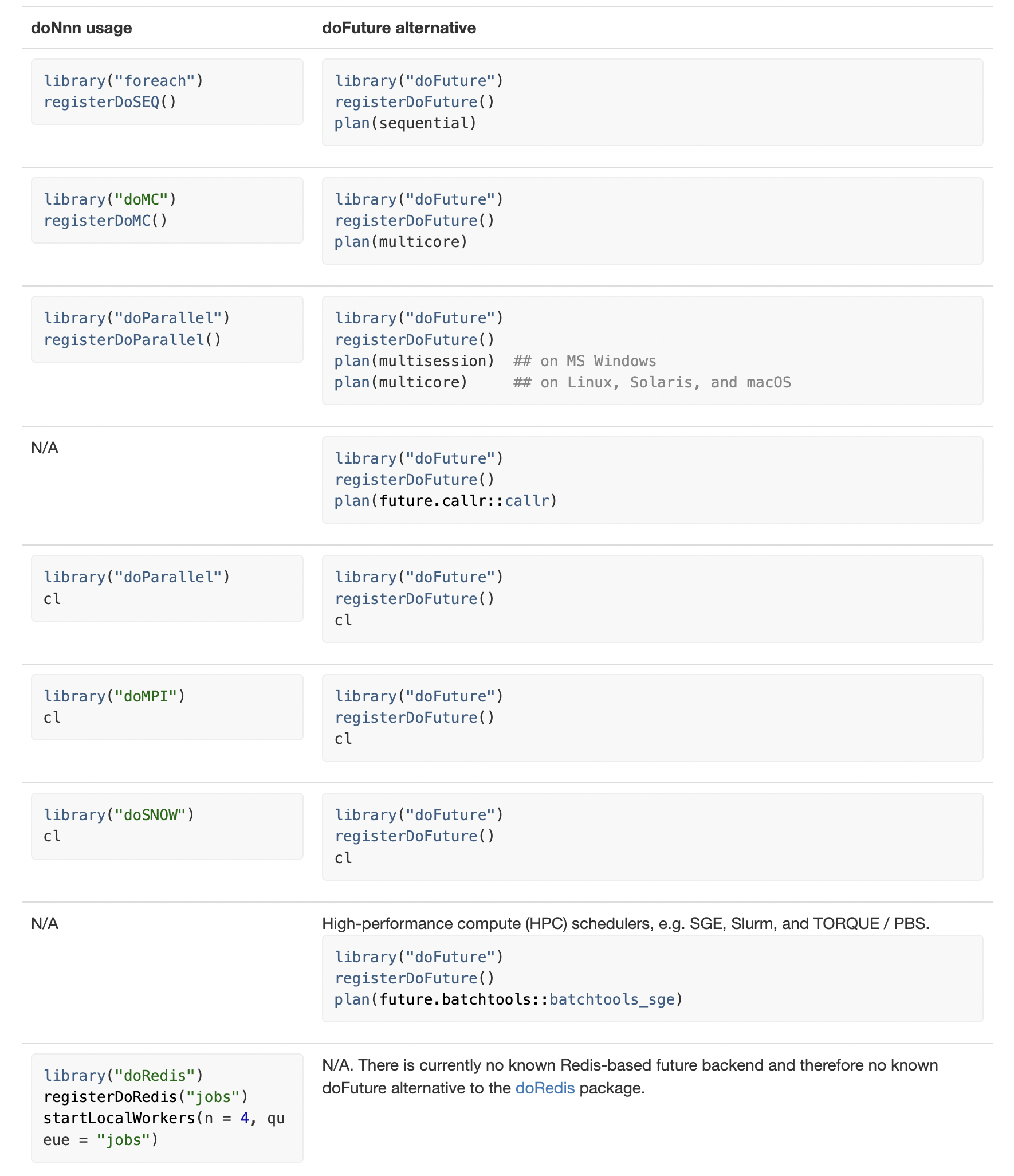
[1] "Running i = 8 in process: 5151"

toc()

1.44 sec elapsed

In the passed, to use foreach with more varied parallel backends you we need to use additional specialised packages. Due to the generic nature of futures, the doFuture package provides the same functionality as many of the existing doNnn packages combined, e.g. doMC, doParallel, doMPI, and doSNOW.

`doFuture` replaces existing `doNnn` packages

As mentioned, a nice feature of using the futureverse is that environment configuration of child processes happen automatically without having to explicitly pass names of packages and objects.

foreach(file = c("abc.txt", "def.log")) %dopar% file_ext(file)

[[1]]
[1] "txt"

[[2]]
[1] "log"

Task parallel problems

All the examples we’ve discussed above refer to data parallel problems which perform the same operation on subsets of the input data. These are the most common examples of embarassingly parallel problems and often the easiest to parallelise.

However, they are not the only type of problem that can be parallelised. Another type of parallelism involves task parallelism.

Task Parallelism refers to the concurrent execution of different task across multiple executing units. Again these maybe cores within a CPU, maybe multiple CPUs (possibly each with multiple cores), and maybe multiple computers systems. Inputs to the differing operations maybe the same but can also be different data.

Let’s look at the differences between data and task parallelism:

Data parallelism vs. task parallelism
Data parallelism	Task parallelism
Same operations are performed on different subsets of same data.	Different operations are performed on the same or different data.
Synchronous computation	Asynchronous computation
Speedup is more as there is only one execution thread operating on all sets of data.	Speedup is less as each processor will execute a different thread or process on the same or different set of data.
Amount of parallelization is proportional to the input data size.	Amount of parallelization is proportional to the number of independent tasks to be performed.

Examples of task parallel problems:

Pre-processing different sources of data before being able to combine and analyse.
Applying different algorithms to a single satellite images to detect separate feature.

Task parallelisms and futures

A way to deploy task parallelism is through the concept of futures.

In programming, a future is an abstraction for a value that may be available at some point in the future. The state of a future can either be unresolved or resolved. As soon as it is resolved, the value is available instantaneously.

If the value is queried while the future is still unresolved by a process that requires it to proceed, the process blocked until the future is resolved.

Exactly how and when futures are resolved depends on what strategy is used to evaluate them. For instance, a future can be resolved using a sequential strategy, which means it is resolved in the current R session. Other strategies may be to resolve futures asynchronously, for instance, by evaluating expressions in parallel on the current machine or concurrently on a compute cluster.

The purpose of the future package, which forms the basis of the futureverse, is to provide a very simple and uniform way of evaluating R expressions asynchronously.

By assigning expressions to asynchronous futures, the current/main R process does not block, which means it is available for further processing while the futures are being resolved in separate processes running in the background. In other words, futures provide a simple yet powerful construct for parallel and / or distributed processing in R.

Let’s expand our example to see how we can use futures to perform task parallelisation.

Let’s write two functions that each perform something slightly different:

example_fun1() goes to sleep for 1 second and then returns a data.frame containing the value of i, the pid (process ID) and the result of i + 10
example_fun2() does something very similar but goes to sleep for 2 seconds while result is the result of i + 20.

example_fun1 <- function(i) {
    Sys.sleep(1)  ## Do nothing for 1 second
    data.frame(i = i, pid = Sys.getpid(), result = i + 10)  
}

example_fun2 <- function(i) {
    Sys.sleep(2)  ## Do nothing for 2 second
    data.frame(i = i, pid = Sys.getpid(), result = i + 20)  
}

Let’s imagine these function represent different pre-processing that needs to be done to data before we can analyse it. In the example analytical workflow below, we start by creating some data, a sequence of integers of length n_cores/2.

The next part of the workflow performs the pre-processing of each element of our data data using lapply and cbind to combine the results into a data.frame. The script first performs the pre-processing using example_fun1 to create processed_data_1 and afterwards performs the pre-processing using example_fun2 to create processed_data_2. Each step happens sequentially.

Finally, the analysis of our processed data is represented by the sum of the values in the results column of processed_data_1 & processed_data_2.

data <- 1:(n_cores/2)
data

[1] 1 2 3 4

tic()
# Pre-processing of data
processed_data_1 <- do.call(rbind, lapply(data, example_fun1))
processed_data_2 <- do.call(rbind, lapply(data, example_fun2))

# Analysis of data
sum(processed_data_1$result, processed_data_2$result)

[1] 140

toc()

12.069 sec elapsed

processed_data_1

  i  pid result
1 1 4098     11
2 2 4098     12
3 3 4098     13
4 4 4098     14

processed_data_2

  i  pid result
1 1 4098     21
2 2 4098     22
3 3 4098     23
4 4 4098     24

We can see that all operations were carried out by the same process sequentially, taking a total of ~ length(data) * 1 + length(data) * 2 = `r length(data) * 1 + length(data) * 2` seconds.

Using `future` & `%<-%` to parallelise independent tasks

What we could do to speed up the execution of our code would be to parallelise the pre-processing step of our analysis. To do this we have use the future package to create processed_data_1 and processed_data_2 as futures that can be evaluated in parallel. To do so we use the %<-% operator instead of the standard <- operator.

library(future)
plan(sequential)

tic()
processed_data_1 %<-% do.call(rbind, lapply(data, example_fun1))
processed_data_2 %<-% do.call(rbind, lapply(data, example_fun2))

sum(processed_data_1$result, processed_data_2$result)

[1] 140

toc()

12.075 sec elapsed

processed_data_1

  i  pid result
1 1 4098     11
2 2 4098     12
3 3 4098     13
4 4 4098     14

processed_data_2

  i  pid result
1 1 4098     21
2 2 4098     22
3 3 4098     23
4 4 4098     24

If we run our futures version using a sequential execution plan, we see the same behaviour as we did without using futures.

However, let’s have a look at what happens when specify a multisession execution plan:

plan(multisession)

tic()
processed_data_1 %<-% do.call(rbind, lapply(data, example_fun1))
processed_data_2 %<-% do.call(rbind, lapply(data, example_fun2))

sum(processed_data_1$result, processed_data_2$result)

[1] 140

toc()

8.129 sec elapsed

processed_data_1

  i  pid result
1 1 5546     11
2 2 5546     12
3 3 5546     13
4 4 5546     14

processed_data_2

  i  pid result
1 1 5554     21
2 2 5554     22
3 3 5554     23
4 4 5554     24

We can see that processed_data_1 and processed_data_2 were created in different processes in parallel and that the whole operation now took ~ length(data) * 2 = 8 seconds, i.e. the time it took for the slowest task to execute.

Combining data and task parallelism

Given that the lapply call is also amenable to data parallelism, we can go a step further and combine task and data parallelism in our execution plan. This will involve nested paralellisation, where the futures are initially parallelised and within each, execution of lapply is also parallelised. To do this we need two things:

swap our our lapplys with future_lapplys.
create a nested execution plan and allocate the correct number of workers to each. To do so we provide a list containing the evaluation strategy we want at each level of nestedness. To be able to set the appropriate number of workers on each one, we also wrap each evaluation strategy definition in function tweak() which allows us to override the default values.

Let’s give it a go!

plan(list(tweak(multisession, workers = 2), 
          tweak(multisession, workers = n_cores/2)))

tic()
processed_data_1 %<-% do.call(rbind, future_lapply(data, example_fun1))
processed_data_2 %<-% do.call(rbind, future_lapply(data, example_fun2))

sum(processed_data_1$result, processed_data_2$result)

[1] 140

toc()

2.892 sec elapsed

processed_data_1

  i  pid result
1 1 6041     11
2 2 6043     12
3 3 6040     13
4 4 6042     14

processed_data_2

  i  pid result
1 1 6160     21
2 2 6161     22
3 3 6159     23
4 4 6158     24

As you can see, each result value in each processed data.frame was computed in parallel in a completely separate process! And now our whole computation executes in ~ 3 secs, the time it takes to run a single iteration of the slowest function plus some overhead to handle the complexity of the execution plan. All in all that’s a nice speed up from our original 12 seconds!

Let’s wrap up and close down any parallel workers

plan(sequential)

Take aways

There is a large number of approaches for tackling parallel computation in R.
Approaches have been evolving over time towards separating the act of writing code that can be executed in parallel when developing from the specification of the specification of parallel backends during runtime.
The most recent and unified approach is that provided by the futureverse ecosystem of packages which is also seeing the most development. The ecosystem provides parallel drop in replacements for many common R programming styles meaning you can stick to your preferred style when parallelising.
The most common and easiest tasks to parallelise are those representing data parallel problems. However, futures also offers options for task parallelisation.

Embarassingly parallel problems

Data parallel problems

Examples of data parallel problems:

Map-reduce parallel programming

Parallel computing in R

Data parallel map-reduce problems

parallel package

mclapply()

parLapply()

foreach package

Combining results

Error handling

Environment management

The futureverse

Execution plan specification in the futureverse

future.apply package

furrr package

foreach using doFuture backend

doFuture replaces existing doNnn packages