Benchmarking

Benchmarking effectively refers to timing execution of our code, although aspects of memory utilisation can also be compared during benchmarking.

There are many ways to benchmark code in R and here we’ll review some of the most useful ones.

Simple benchmarking

`system.time()`

The function takes an expression and returns the CPU time used to evaluate the expression. It is a primitive function and part of base R an a good starting point for timing R expressions.

system.time(
    for(i in 1:100) mad(runif(1000))
    )

   user  system elapsed 
  0.007   0.001   0.007

The output prints a named vector of length 3.

The first two entries are the total user and system CPU times of the current R process and any child processes on which it has waited, and the third entry is the ‘real’ elapsed time since the process was started.

The resolution of the times will be system-specific.

Expressions across multiple lines can be run by enclosing them in curly braces ({}).

system.time({
    for(i in 1:100) {
        v <- runif(1000)
        mad(v)
    }
})

   user  system elapsed 
  0.007   0.001   0.008

`tictoc` 📦

Package tictoc provides similar functionality to system.time with some additional useful features. To time code execution, you can wrap them between function calls tic and toc.

library(tictoc)

tic()

for (i in 1:100) {
    v <- runif(1000)
    mad(v)
}

toc()

0.008 sec elapsed

The nice features of the tictoc package is that;

Descriptive messages can be associated with each timing through tic argument msg.
Timings can be nested.
Timings can be logged through toc argument log = TRUE and accessed afterwards through tic.log().

tic(msg = "MAD 100 iterations of 1000 random values")

for (i in 1:100) {
    v <- runif(1000)
    mad(v)
}

toc(log = TRUE)

MAD 100 iterations of 1000 random values: 0.008 sec elapsed

tic(msg = "MAD 1000 iterations of 1000 random values")

for (i in 1:1000) {
    v <- runif(1000)
    mad(v)
}

toc(log = TRUE)

MAD 1000 iterations of 1000 random values: 0.067 sec elapsed

tic(msg = "MAD 100 iterations of 10000 random values")

for (i in 1:100) {
    v <- runif(10000)
    mad(v)
}

toc(log = TRUE)

MAD 100 iterations of 10000 random values: 0.044 sec elapsed

tic.log()

[[1]]
[1] "MAD 100 iterations of 1000 random values: 0.008 sec elapsed"

[[2]]
[1] "MAD 1000 iterations of 1000 random values: 0.067 sec elapsed"

[[3]]
[1] "MAD 100 iterations of 10000 random values: 0.044 sec elapsed"

Formal Benchmarking

system.time() and tictoc are straightforward and simple to use for timing individual of code. However, there do have a few limitations:

They only time execution time of the code once. As we’ve seen there’s a lot of other things going on on your system which may affect execution time at any one time. So timings can vary if tested repeatedly.
Comparing different expressions has to be performed rather manually, especially if we want to also check expressions being compared give the same result.

There are a number of packages in R that make benchmarking code, especially the comparison of different expressions much easier and robust. Here we will explore two of these, microbenchmark and bench.

`microbenchmark` 📦

The microbenchmark() function in package microbenchmark serves as a more accurate replacement of system.time(). To achieved this, the sub-millisecond (supposedly nanosecond) accurate timing functions most modern operating systems provide are used. This allows us to compare expressions with much shorter execution times.

Some nice package features:

By default evaluates each expression multiple times, by default 100 but this number can be controlled through argument times.
You can enforce checks on the results to ensure each expression tested returns the same result, with various levels of strictness through argument check.
You can supply setup code that will be run by each iteration without contributing to the timing through argument setup.
Note that the function is only meant for micro-benchmarking small pieces of source code and to compare their relative performance characteristics.

See the function documentation for more info.

Let’s go ahead and look at an example.

Centering data in data.frame by column mean

Let’s say we are given the following code and asked to speed it up.

In this example, first a data frame is created that has 151 columns. One of the columns contains a character ID, and the other 150 columns contain numeric values.

For each numeric column, the code calculates the mean and subtracts it from the values in the column, so the data in each column is centered on the mean.

rows <- 400000
cols <- 150
data <- as.data.frame(x = matrix(rnorm(rows * cols, mean = 5), ncol = cols))
data <- cbind(id = paste0("g", seq_len(rows)), data)

# Get column means
means <- apply(data[, names(data) != "id"], 2, mean)

# Subtract mean from each column
for (i in seq_along(means)) {
    data[, names(data) != "id"][, i] <- data[, names(data) != "id"][, i] - means[i]
}

Looking at it, we might think back to the age old R advice to “avoid loops”. So to improve performance of our code we might start by working on the for loop.

Let’s use microbenchmark to test the execution times of alternative approaches and compare them to the original approach:

Give we we want to iterate across more than one objects (means and the columns in our data) might consider the mapply function. We then reassign the result back to the appropriate columns in our data.frame.
We could also try purrrs map2_dfc which takes two inputs and column binds the results into a data.frame. We can again reassign the result back to the appropriate columns in our data.frame.

To test out our approaches we might want to make a smaller version of our data to work with. Let’s create a smaller data frame with 40,000 rows and 50 columns and re-calculate our means vector:

rows <- 40000
cols <- 50
data <- as.data.frame(x = matrix(rnorm(rows * cols, mean = 5), ncol = cols))
data <- cbind(id = paste0("g", seq_len(rows)), data)

means <- apply(data[, names(data) != "id"], 2, mean)

Now let’s wrap our original for loop and our two test approaches in a benchmark.

We can wrap each expression in {} and pass it as a named argument for easier review of our benchmark results.

Let’s only run 50 iterations instead of the default 100 through argument times.

Let’s also include some setup code so that a new data_bnch object is created before each benchmark expression so that we don’t overwrite the data object in the global environment.

microbenchmark::microbenchmark(
    for_loop = {
        for (i in seq_along(means)) {
            data_bnch[, names(data_bnch) != "id"][, i] <- 
                data_bnch[, names(data_bnch) != "id"][, i] - means[i]
        }
    }, 
    mapply = {
        data_bnch[, names(data_bnch) != "id"] <- mapply(
            FUN = function(x, y) x - y,
            data_bnch[, names(data_bnch) != "id"], 
            means)
    },
      map2_dfc = {
        data_bnch[, names(data_bnch) != "id"] <- purrr::map2_dfc(
                            data_bnch[, names(data_bnch) != "id"], 
                            means, 
                            ~.x - .y)
    },
    times = 50,
    setup = {data_bnch <- data}
)

Warning in microbenchmark::microbenchmark(for_loop = {: less accurate nanosecond
times to avoid potential integer overflows

Unit: milliseconds
     expr       min        lq     mean    median        uq       max neval cld
 for_loop 11.509684 11.807836 13.25639 12.314801 14.811496  17.67621    50  a 
   mapply 38.608306 42.438239 55.66920 45.157359 73.807093 114.07528    50   b
 map2_dfc  3.237155  3.783111 11.45792  3.922573  5.906091 215.98726    50  a

The results of our benchmark return one row per expression tested.

expr contains the name of the expression.
min, lq, mean, median, uq and max are summary statistics of the execution times across all iterations.
neval shows the numbers of iterations

So far, purrr::map2_dfc() is looking like the best option.

But are we sure we are getting the same results form each approach?

To ensure this we can re-run our benchmarks using the check argument. A value of "equal" will compare all values output by the benchmark using all.equal(). For the comparison to work, we need the last expression of the computation to output the same object. As this differs in the for loop from the two others, we include a call to print the final object data_bnch for comparison in each expression.

microbenchmark::microbenchmark(
    for_loop = {
        for (i in seq_along(means)) {
            data_bnch[, names(data_bnch) != "id"][, i] <- 
                data_bnch[, names(data_bnch) != "id"][, i] - means[i]
        }
        data_bnch
    }, 
    mapply = {
        data_bnch[, names(data_bnch) != "id"] <- mapply(
            function(x, y) x - y,
            data_bnch[, names(data_bnch) != "id"], 
            means)
        data_bnch
    },
      map2_dfc = {
        data_bnch[names(data_bnch) != "id"] <- purrr::map2_dfc(
                            data_bnch[, names(data_bnch) != "id"], 
                            means, 
                            ~.x - .y)
        data_bnch
    },
    times = 50,
    setup = {data_bnch <- data},
    check = "equal"
)

Unit: milliseconds
     expr       min        lq      mean    median       uq       max neval cld
 for_loop 10.800794 11.518171 15.133487 11.725980 12.10574  81.62780    50  b 
   mapply 36.060894 41.134193 55.993229 43.386958 45.70668 118.76507    50   c
 map2_dfc  2.813543  3.505951  6.105265  3.841167  5.78838  76.05471    50 a

Excellent! We can now be confident that our tests are retuning the same result.

Finally, if you like to compare things visually, the output of our benchmark can be provided as an input to the autoplot.microbenchmark method to produce a graph of microbenchmark timings.

library(ggplot2)
library(dplyr)
microbenchmark::microbenchmark(
    for_loop = {
        for (i in seq_along(means)) {
            data_bnch[, names(data_bnch) != "id"][, i] <- 
                data_bnch[, names(data_bnch) != "id"][, i] - means[i]
        }
        data_bnch
    }, 
    mapply = {
        data_bnch[, names(data_bnch) != "id"] <- mapply(
            function(x, y) x - y,
            data_bnch[, names(data_bnch) != "id"], 
            means)
        data_bnch
    },
      map2_dfc = {
          data_bnch[names(data_bnch) != "id"] <- purrr::map2_dfc(
                            data_bnch[, names(data_bnch) != "id"], 
                            means, 
                            ~.x - .y)
        data_bnch
    },
    times = 50,
    setup = {data_bnch <- data},
    check = "equal"
) %>%
autoplot()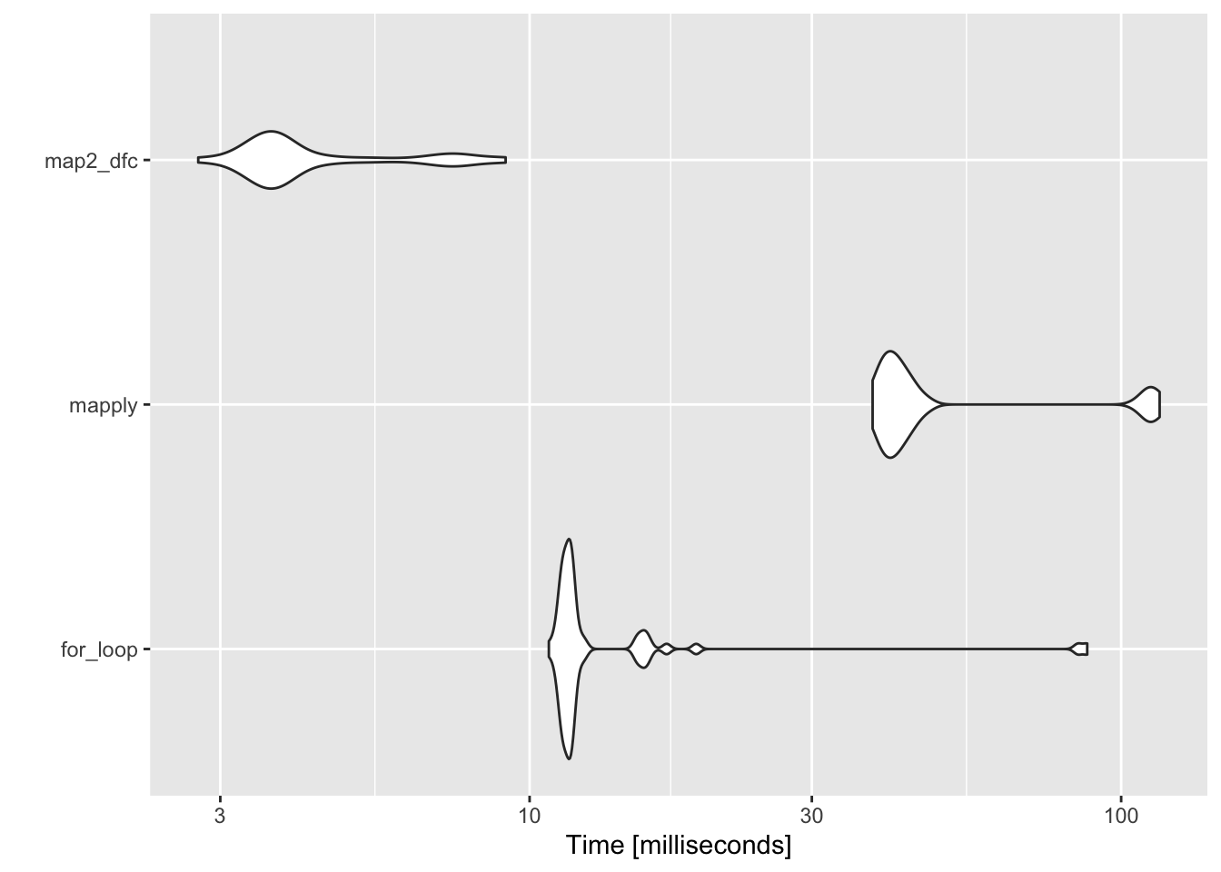

`bench` 📦

bench is similar to microbenchmark. However it offers some additional features which means I generally prefer it.

The main function equivalent to microbenchmark() is mark().

`mark()`

PROs

The main pro in my view is that it also tracks memory allocations for each expression.
It also tracks the number and type of R garbage collections per expression iteration.
It verifies equality of expression results by default, to avoid accidentally benchmarking inequivalent code.
It allows you to execute code in separate environments (so that objects in global environment are not modified).

Some cons to consider:

it doesn’t have a setup option.
the output object, while much more informative than that of microbenchmark can be quite bloated itself.

So let’s go ahead and run our tests using bench::mark().

Because there is no setup option, we need to create data_bnch at the start of each expression. We can also use argument env = new.env() to perform all our computation in a separate environment.

Because mark() checks for equality by default, we use the version of our expressions that print the resulting data_bnch at the end for comparison.

bench::mark(
    for_loop = {
        data_bnch <- data
        for (i in seq_along(means)) {
            data_bnch[, names(data_bnch) != "id"][, i] <- 
                data_bnch[, names(data_bnch) != "id"][, i] - means[i]
        }
        data_bnch
    }, 
    mapply = {
        data_bnch <- data
        data_bnch[, names(data_bnch) != "id"] <- mapply(
            function(x, y) x - y,
            data_bnch[, names(data_bnch) != "id"], 
            means)
        data_bnch
    },
      map2_dfc = {
          data_bnch <- data
          data_bnch[names(data_bnch) != "id"] <- purrr::map2_dfc(
                            data_bnch[, names(data_bnch) != "id"], 
                            means, 
                            ~.x - .y)
        data_bnch
    },
    env = new.env()
)

Warning: Some expressions had a GC in every iteration; so filtering is disabled.

# A tibble: 3 × 6
  expression      min   median `itr/sec` mem_alloc `gc/sec`
  <bch:expr> <bch:tm> <bch:tm>     <dbl> <bch:byt>    <dbl>
1 for_loop     9.33ms  10.11ms      84.9    17.4MB     19.3
2 mapply      37.69ms  42.43ms      16.9   138.1MB     28.1
3 map2_dfc     2.66ms   3.49ms     251.     15.3MB     29.6

Let’s have a look at the output in detail:

expression - bench_expr The deparsed expression that was evaluated (or its name if one was provided).
min - The minimum execution time.
median - The sample median of execution time.
itr/sec - The estimated number of executions performed per second.
mem_alloc - Total amount of memory allocated by R while running the expression.
gc/sec - The number of garbage collections per second.
n_itr - Total number of iterations after filtering garbage collections (if filter_gc == TRUE).
n_gc - Total number of garbage collections performed over all iterations.
total_time - The total time to perform the benchmarks.
result - list A list column of the object(s) returned by the evaluated expression(s).
memory - list A list column with results from Rprofmem().
time - list A list column of vectors for each evaluated expression.
gc - list A list column with tibbles containing the level of garbage collection (0-2, columns) for each iteration (rows).

I find the addition of the mem_alloc particularly useful. Just look at the difference between mapply and the other two approaches in term of memory usage!

As you can see, there’s a lot more information in the bench::mark() output. Note as well there are a number of list columns at the which include results of the evaluated expressions, results of Rprofmem() and a list of garbage collection events. This can be quite useful to dig into.

However, if this object is assigned to a variable or you try to save it, it could take up A LOT of space depending on the size of the results and number of internal calls. So I recommend getting rid of such columns if you want to save benchmarks.

`press()`

Another cool feature of the bench package is bench::pressing() using the press() function. press() can be used to run mark() across a grid of parameters and then press the results together.

We set the parameters we want to test across as named arguments and a grid of all possible combinations is automatically created.

The code to setup the benchmark is passed as a single unnamed expression before calling the bench::mark() code we want to run with the grid of parameters.

Let’s have a look at how this works.

Say we want to test the performance of our three approaches on data.frames of different sizes varying both rows and columns.

We can specify two parameters in bench::press() as named arguments rows and columns and assigns vectors of the values we want press() to create a testing grid from.

The next curly braces {} contain our setup code which create data.frames of different sizes and the benchmark.

bp <- bench::press(
    rows = c(1000, 10000, 400000),
    cols = c(10, 50, 100),
    {
        {
            # Bench press setup code:
            # create data.frames of different sizes using parameters 
            # rows & columns
            set.seed(1)
            data <- as.data.frame(x = matrix(
                rnorm(rows * cols, mean = 5), 
                ncol = cols))
            data <- cbind(id = paste0("g", seq_len(rows)), data)
            means <- apply(data[, names(data) != "id"], 2, mean)
        }
        bench::mark(
            for_loop = {
                data_bnch <- data
                for (i in seq_along(means)) {
                    data_bnch[, names(data_bnch) != "id"][, i] <- 
                        data_bnch[, names(data_bnch) != "id"][, i] - means[i]
                }
                data_bnch
            }, 
            mapply = {
                data_bnch <- data
                data_bnch[, names(data_bnch) != "id"] <- mapply(
                    function(x, y) x - y,
                    data_bnch[, names(data_bnch) != "id"], 
                    means)
                data_bnch
            },
            map2_dfc = {
                data_bnch <- data
                data_bnch[names(data_bnch) != "id"] <- purrr::map2_dfc(
                    data_bnch[, names(data_bnch) != "id"], 
                    means, 
                    ~.x - .y)
                data_bnch
            },
            env = new.env(),
            time_unit = "us"
        )
    }
)

Running with:
    rows  cols

1   1000    10

2  10000    10

3 400000    10

Warning: Some expressions had a GC in every iteration; so filtering is disabled.

4   1000    50

5  10000    50

6 400000    50

Warning: Some expressions had a GC in every iteration; so filtering is disabled.

7   1000   100

8  10000   100

9 400000   100

Warning: Some expressions had a GC in every iteration; so filtering is disabled.

bp

# A tibble: 27 × 8
   expression   rows  cols    min  median `itr/sec` mem_alloc `gc/sec`
   <bch:expr>  <dbl> <dbl>  <dbl>   <dbl>     <dbl> <bch:byt>    <dbl>
 1 for_loop     1000    10   555.    572.   1736.     78.87KB     25.8
 2 mapply       1000    10   216.    257.   3915.    754.36KB     17.9
 3 map2_dfc     1000    10  1350.   1562.    622.     82.87KB     10.5
 4 for_loop    10000    10   572.    626.   1610.    781.99KB     24.4
 5 mapply      10000    10  1547.   1956.    522.      7.11MB     20.7
 6 map2_dfc    10000    10  1484.   1629.    600.    785.99KB     10.6
 7 for_loop   400000    10  2026.   3094.    135.     30.52MB     49.8
 8 mapply     400000    10 85374. 131481.      7.43  276.14MB     18.6
 9 map2_dfc   400000    10  2857.   4572.    146.     30.52MB     20.0
10 for_loop     1000    50  8618.   8847.    113.      2.52MB     13.1
# … with 17 more rows

Now when we look at our benchmark we see we get results for each approach and also for each row x column combination.

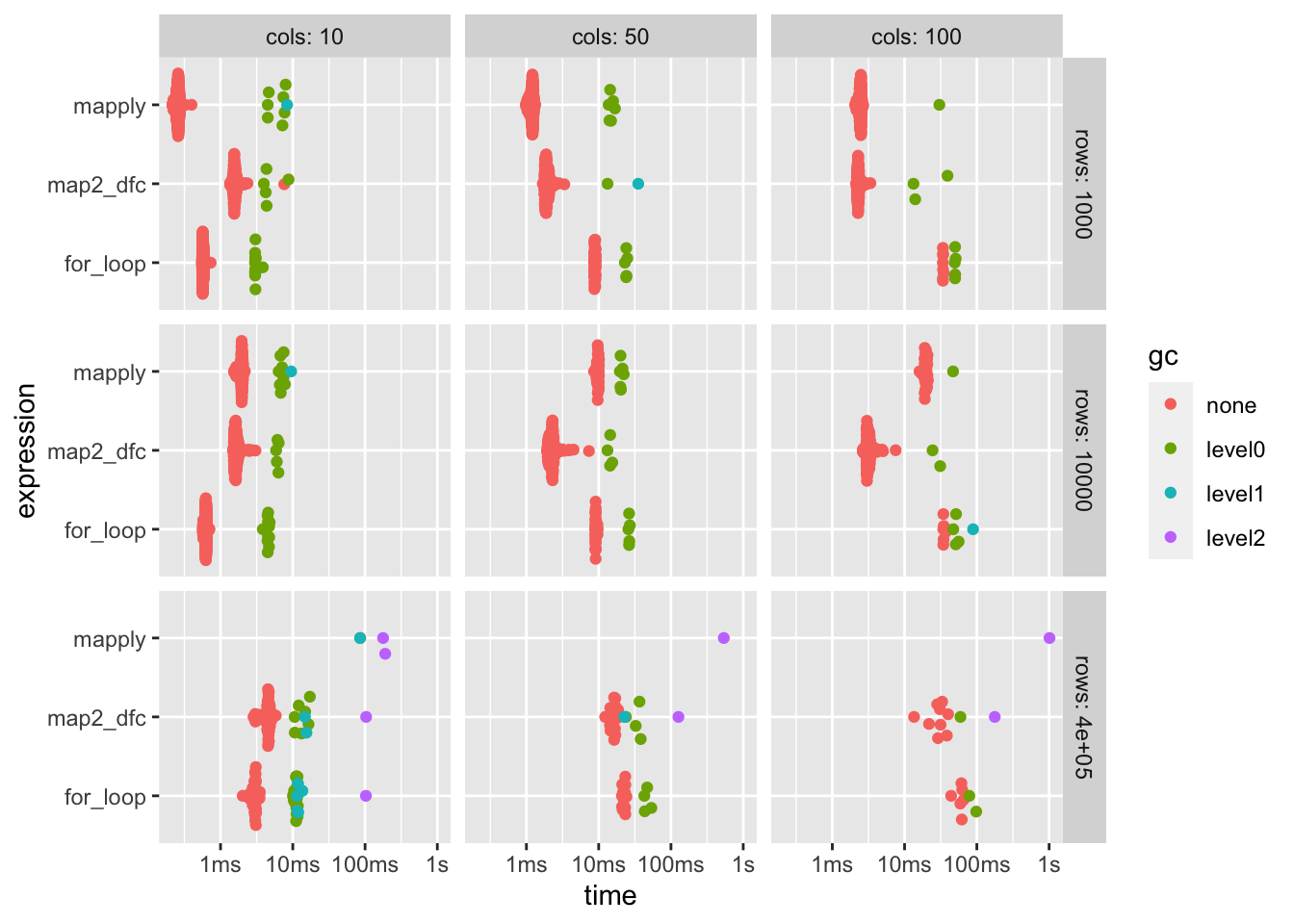
Let’s plot the results again using autoplot to get a better overview of our results

autoplot(bp)

Loading required namespace: tidyr

What thus show is that:

for the smallest data.frame sizes, mapply is actually quite performant!
for loops are also fastest when the number of columns is small regardless of number of rows.
map2_dfc becomes the better performer as number of columns increases.

Simple benchmarking

system.time()

tictoc 📦

Formal Benchmarking

microbenchmark 📦