Best practice for writing efficient code

We’ve had a look at ways to benchmark your code and identify bottlenecks. When making optimisation decisions, it’s always best to use theses tools to be get hard data on how your code is likely to perform. Having said that, there are some golden rules in R programming that can help you write performant code from the start and help guide the search for more efficient solutions when bottlenecks are identified.

In the next few sections, we’ll have a look at some key best practices for writing efficient R code. A characteristic of R is that there are many many ways to do the same thing. We will look at a lot of examples here that might seem like a strange way to do things, and many are! However, it’s often quite instructive to benchmark and memory profile such code to make what’s going on more concrete.

Let’s start with one of the most pernicious drain on performance which should be avoided at all costs, growing data structures!

Avoid growing data structures

Let’s start with an example vector x of 1000 random numbers between 1 and 100.

set.seed(20230116)
x <- runif(10000, min = 1, max = 100)

Let’s say we want to process our vector with a simple algorithm. If the value of x is less that 10, recode to 0. Otherwise, take the square root.

library(dplyr)
library(pryr)
library(ggplot2)

The perils of growing data structures

The most basic implementation we might think of is a for loop that processes each element individually, using an if statement to decide what action to take depending on the value of the element and appending the processed output of each iteration using the c() function, element by element, to another vector y.

Let’s create a function to implement it:

for_loop_c <- function(x) {
    y <- NULL
    for (i in seq_along(x)) {
        if (x[i] < 10) {
            y <- c(y, 0)
        } else {
            y <- c(y, sqrt(x[i]))
        }
    }
    y
}

Let’s go ahead and make a starting benchmark:

bench::mark(
    for_loop_c(x)
)

Warning: Some expressions had a GC in every iteration; so filtering is disabled.

# A tibble: 1 × 6
  expression         min   median `itr/sec` mem_alloc `gc/sec`
  <bch:expr>    <bch:tm> <bch:tm>     <dbl> <bch:byt>    <dbl>
1 for_loop_c(x)   97.8ms    102ms      9.67     382MB     87.0

It might not seem obvious until we start comparing it to other approaches but this is actually very slow for processing a numeric vector of length 10000. Notice as well how much memory is allocated to the execution, especially compared to the size of the original vector!

object_size(x)

80.05 kB

The biggest problem with this implementation, and the reason for loops are so often (wrongly) maligned for inefficiency is the fact that we are incrementally growing the result vector y using function c.

To dig into the issue let’s contrast it to another approach for growing vectors, using sub-assignment.

In the following example, we’re doing the same processing to each element but instead of binding it to y using c(), we use sub-assignment to increment the length of y directly.

for_loop_assign <- function(x) {
    y <- NULL
    for (i in seq_along(x)) {
        if (x[i] < 10) {
            y[i] <- 0
        } else {
            y[i] <- sqrt(x[i])
        }
    }
    y
}

Let’s compare the two approaches with a benchmark.

bench::mark(
    for_loop_c(x),
    for_loop_assign(x)
)

Warning: Some expressions had a GC in every iteration; so filtering is disabled.

# A tibble: 2 × 6
  expression              min   median `itr/sec` mem_alloc `gc/sec`
  <bch:expr>         <bch:tm> <bch:tm>     <dbl> <bch:byt>    <dbl>
1 for_loop_c(x)      104.71ms 110.33ms      9.12     382MB     82.1
2 for_loop_assign(x)   1.24ms   1.32ms    654.       1.7MB     30.0

That’s a big difference! We’re still growing the vector element by element in for_loop_assign, but it’s much faster than using the c() function. It’s also much more memory efficient! Why?

Well, to get to the bottom of this, I actually ended up posting a question on stack overflow. Let’s investigate with an experiment. I’ve created adapted versions of the functions that perform a simplified version of the element-wise processing but also record the cumulative number of memory address changes at each iteration.

If the address of y in any given iteration is not the same as the previous one, the cumulative count of memory addresses that y has occupied during execution is increased. Results are then compiled into a data.frame and cumulative counts and returned instead of y. So the functions now track the number memory addresses changed during our for loop.

# Create function that appends to result vector through c
# Collect cumulative number of address changes per iteration
for_loop_c_addr <- function(x, count_addr = TRUE) {
    y <- NULL
    y_addr <- address(y)
    cum_address_n <- 0
    cum_address_n_v <- numeric(length(x))

    for (i in seq_along(x)) {
        y <- c(y, sqrt(x[i]))
            if (address(y) != y_addr) {
                cum_address_n <- cum_address_n + 1
                y_addr <- address(y)
            }

        cum_address_n_v[i] <- cum_address_n
    }
    data.frame(i = seq_along(cum_address_n_v),
               cum_address_n = cum_address_n_v,
               mode = "c")
}

# Create function that appends to result vector through assignment.
# Collect cumulative number of address changes per iteration
for_loop_assign_addr <- function(x) {
    y <- NULL
    y_addr <- address(y)
    cum_address_n <- 0
    cum_address_n_v <- numeric(length(x))

    for (i in seq_along(x)) {

        y[i] <- sqrt(x[i])
            if (address(y) != y_addr) {
                cum_address_n <- cum_address_n + 1
                y_addr <- address(y)
            }
        cum_address_n_v[i] <- cum_address_n
    }
    data.frame(i = seq_along(cum_address_n_v),
               cum_address_n = cum_address_n_v,
               mode = "assign")
}

## Execute function, compile results and plot
c_df <- for_loop_c_addr(x)
assign_df <- for_loop_assign_addr(x)

We can now explore our results by are plotting the cumulative count of address changes against i.

Let’s have a look at what happens during sub-assignment:

assign_df |>
    ggplot(aes(x = i, y = cum_address_n, colour = mode)) +
    geom_line() +
    ylab("Cumulative count of address changes")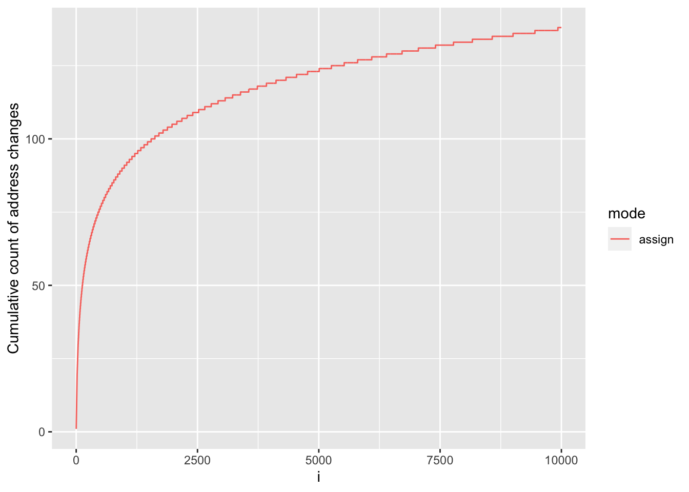

We see that, although address changes throughout our for loop as a result of memory requests to accommodate the growing vectors, this does not occur at every iteration, in fact it happens a total of 138 times. In between these events, y is being grown in-place without needing to change address.

This occurs because, since version 3.4.0, R will allocate a bit of extra memory for atomic vectors when requesting additional memory, so that ‘growing’ such vectors via sub-assignment may not require a reallocation if some spare capacity is still available, and indeed that’s what we see in our experiment.

Let’s know plot it against our results for the c() approach:

rbind(c_df, assign_df) |>
    ggplot(aes(x = i, y = cum_address_n, colour = mode)) +
    geom_line() +
    ylab("Cumulative count of address changes")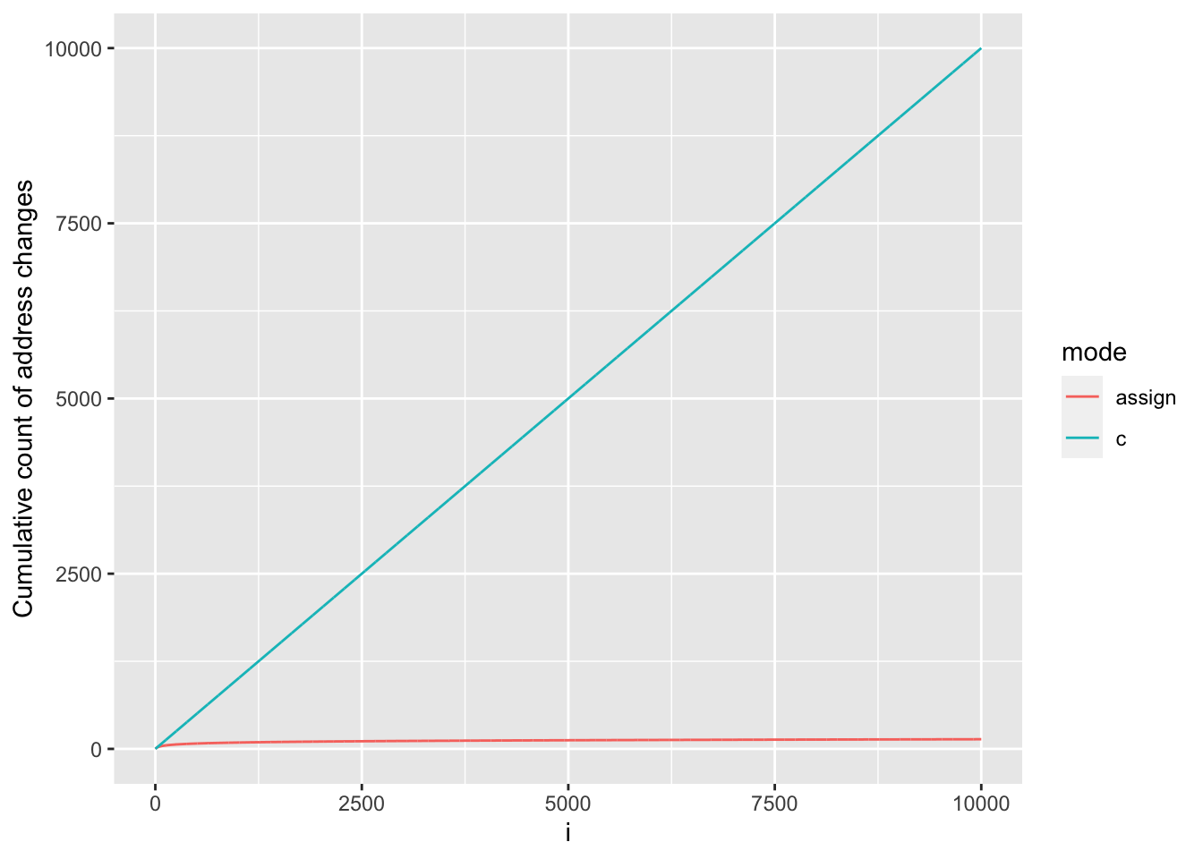

When using c(), R must first allocate space for the new y created by the output of c() and then copy the inputs to c() (i.e. previous y and the additional value being appended) object to its new memory location. This results in a change of address at every iteration. Because requests for additional memory are costly, using c() to grow a results vector is so much slower and memory inefficient.

The same is true for functions like c(), append(), cbind(), rbind(), or paste() so avoid using them in a for loop at all costs.

Pre-allocating data structures

The best way to improve the performance of our algorithm is to pre allocate a results vector of the required size and then assign our results to elements that already exist. This allows for R to allocate the required amount for y once and then modify it in place without creating copies at every iteration.

Below I create two functions that do just that. The first one, for_loop_preallocate_NA() creates a vector of NAs the same length as x whereas the second function for_loop_preallocate_num() creates a numeric vector.

for_loop_preallocate_NA <- function(x) {
    y <- rep(NA, times = length(x))
    
        for (i in seq_along(x)) {
            if (x[i] < 10) {
                y[i] <- 0
            } else {
                y[i] <- sqrt(x[i])
            }
        }
        y
}

for_loop_preallocate_num <- function(x) {
    y <- numeric(length = length(x))
    
        for (i in seq_along(x)) {
            if (x[i] < 10) {
                y[i] <- 0
            } else {
                y[i] <- sqrt(x[i])
            }
        }
        y
}

Let’s see what happens to our benchmarks when we pre-allocate the results vector and let’s now look at it in relative terms by using mark() with argument relative = TRUE

bench::mark(
    for_loop_c(x),
    for_loop_assign(x),
    for_loop_preallocate_NA(x),
    for_loop_preallocate_num(x),
    relative = TRUE
)

Warning: Some expressions had a GC in every iteration; so filtering is disabled.

# A tibble: 4 × 6
  expression                     min median `itr/sec` mem_alloc `gc/sec`
  <bch:expr>                   <dbl>  <dbl>     <dbl>     <dbl>    <dbl>
1 for_loop_c(x)               207.   248.         1     3261.      42.7 
2 for_loop_assign(x)            2.72   2.92      80.0     14.2     17.0 
3 for_loop_preallocate_NA(x)    1.03   1.04     241.       1.32     3.00
4 for_loop_preallocate_num(x)   1      1        252.       1        1   

We can see a huge improvement in performance if we pre-allocate y compared to using c() and this is also reflected in the huge drop in memory allocation for the operation.

We also see a very minor speed up and smaller memory foot print by preallocating the appropriate type of vector. This is because in for_loop_preallocate_num() R doesn’t have to coerce y to the appropriate numeric in the first iteration as it does in for_loop_preallocate_NA(), an operation that requires making a copy of the vector.

Another interesting outcome of our benchmarking experiments though is that, since R 3.4.0, growing vectors through sub-assignment can be a reasonable approach if there is no way to know what size object to pre-allocate.

Vectorise as much as possible

Another popular mantra with respect to efficient programming in R to “Vectorise as much as possible”. While it’s indeed another golden rule, it can be a misunderstood concept as I’ve often heard it translated to “Avoid loops, use the apply family instead” which, as you will see, is not actually quite accurate, at least not in many situations.

Let’s for now play along with that interpretation and explore performance of creating custom function cond_sqrt_i() that processes single values and then using some apply and purrr functions (the tidyverse’s answer to the apply family) to apply the function to each element of our vector in one go.

I’ve wrapped two implementations from each family of functions for ease and fairness of comparison to our for loop approaches:

• lapply_unlist_fun() uses lapply and unlist to return a vector of values.

• sapply_fun() uses sapply which returns a vector.

• purrr_map_fun uses the map function from the purrr package and unlist to return a vector.

• purrr_map_dbl_fun uses the map_dbl function fro the purrr package that returns a double vector by default.

cond_sqrt_i <- function(x) {
    if (x < 10) {
        return(0)
    } else {
        return(sqrt(x))
    }
}


lapply_unlist_fun <- function(x) {
    unlist(lapply(x, cond_sqrt_i))
}

sapply_fun <- function(x) {
    sapply(x, cond_sqrt_i)
}

purrr_map_fun <- function(x) {
    unlist(purrr::map(x, cond_sqrt_i))
}

purrr_map_dbl_fun <- function(x) {
    purrr::map_dbl(x, cond_sqrt_i)
}

Let’s go ahead and add these approaches to our benchmarks. I use the dplyr function arrange at the bottom to order the results of our benchmarks by ascending values in median.

bench::mark(
    for_loop_c(x),
    for_loop_assign(x),
    for_loop_preallocate_NA(x),
    for_loop_preallocate_num(x),
    lapply_unlist_fun(x),
    sapply_fun(x),
    purrr_map_fun(x),
    purrr_map_dbl_fun(x),
    relative = TRUE
) %>%
    arrange(median)

Warning: Some expressions had a GC in every iteration; so filtering is disabled.

# A tibble: 8 × 6
  expression                     min median `itr/sec` mem_alloc `gc/sec`
  <bch:expr>                   <dbl>  <dbl>     <dbl>     <dbl>    <dbl>
1 for_loop_preallocate_num(x)   1      1        259.       1        1   
2 for_loop_preallocate_NA(x)    1.03   1.04     221.       1.50     1.50
3 for_loop_assign(x)            2.73   2.95      77.2     21.8      7.99
4 lapply_unlist_fun(x)          5.53   5.78      41.7      2.21     8.43
5 purrr_map_dbl_fun(x)          5.92   6.06      40.4      1.05     8.00
6 purrr_map_fun(x)              6.02   6.19      37.9      6.60     7.97
7 sapply_fun(x)                 5.85   6.27      38.8      4.64     7.50
8 for_loop_c(x)               258.   258.         1     5003.      22.4 

Perhaps the results of this contrived test were surprising, perhaps not. What is clear though is that vectorising your code is not just about avoiding for loops, although that’s often a step.

Yes, vectorised code is more compact and concise, which our latest implementations indeed are. But in the *apply and purrr approaches we tried above, we are not embracing the true concept of vectorisation because we are still having to call if on every element of x and sqrt on many of the element of x. This is pretty much what our original for loop which preallocates the results vector is doing, without the overhead of calling an *apply/purrr function as well.

Vectorising is about taking a whole-object approach to a problem, thinking about vectors, not individual elements of a vector. And to achieve this, we must harness the power of the fact that many many functions in R are themselves vectorised and can take whole vectors as inputs, not just single values, operate on them efficiently and return vectors with a single function call.

Here’s a short list of examples of vectorised operators and functions in R.

• Logical operators: >, <, ==, != etc

• Arithmetic operators: +, -, /, * etc.

• Replacement and indexing operators: [[<-, [<- , [[, [

• Mathematical functions: log(), log10(), exp(), and, fortunately for our example sqrt()!

Under the hood, vectorised functions also implement for loops, but the are performed by C code instead of R code, making them much faster.

Given this, let’s try two more approaches embracing the vectorised nature of (many) R functions:

First, let’s write a function that uses the vectorised ifelse() function. The function takes a logical vector as it’s first argument tests, here created by the comparative statement x < 10 and returns the result of any expression in the second argument yes where elements of test are TRUE and the result of any expression in the third argument no where elements of test are FALSE.

ifelse_fun <- function(x) {
    ifelse(x < 10, 0, sqrt(x))
}

Let’s finally try one last approach making use of both vectorisation and a mathematical trick. We know that the square root of 0 is also zero. With that in mind, we can process x in two vectorised steps, one to convert all values in x < 10 to 0 and then use a single call to sqrt() on the whole vector to get the square root (which will only change the value of non 0 elements).

Tip

Bonus Tip

Sometimes the most effective way to optimise an algorithm or operation is to things carefully about the underlying maths and attempt to optimise through mathematical tricks.

cond_sqrt_vctr <- function(x) {
    x[x < 10] <- 0
    sqrt(x)
}

Let’s do a final benchmark comparing all the approaches we’ve tried:

bench::mark(
    for_loop_c(x),
    for_loop_assign(x),
    for_loop_preallocate_NA(x),
    for_loop_preallocate_num(x),
    lapply_unlist_fun(x),
    sapply_fun(x),
    purrr_map_fun(x),
    purrr_map_dbl_fun(x),
    ifelse_fun(x),
    cond_sqrt_vctr(x),
    relative = TRUE
) %>%
    arrange(median)

Warning: Some expressions had a GC in every iteration; so filtering is disabled.

# A tibble: 10 × 6
   expression                      min  median `itr/sec` mem_alloc `gc/sec`
   <bch:expr>                    <dbl>   <dbl>     <dbl>     <dbl>    <dbl>
 1 cond_sqrt_vctr(x)              1       1       1893.       3.05    22.5 
 2 ifelse_fun(x)                  3.82    3.54     558.       8.00    17.9 
 3 for_loop_preallocate_num(x)   13.9    10.8      254.       1        1   
 4 for_loop_preallocate_NA(x)    14.4    11.2      245.       1.50     1.50
 5 for_loop_assign(x)            38.0    31.7       80.7     21.8      8.50
 6 lapply_unlist_fun(x)          77.5    61.5       41.5      2        7.98
 7 sapply_fun(x)                 80.5    64.4       38.7      4.64     8.96
 8 purrr_map_dbl_fun(x)          82.6    66.8       38.5      1        7.98
 9 purrr_map_fun(x)              85.0    67.9       37.9      2        8.00
10 for_loop_c(x)               3154.   2542.         1     5003.      22.5 

Here we can see that the clear winner in terms of speed, function cond_sqrt_vctr() which harnesses the power of vectorisation most effectively. It’s faster that ifelse because, although ifelse is vectorised, if we look at the source code we see that a big chunk of the body is taken up on performing checks. It also wraps execution of the yes and no expressions in rep() to deal with situations where the expressions themselves cannot be vectorised which adds an additional function call.

Take aways:

• Avoid growing data structures using functions like c(), rbind(), cbind(), append(), paste() etc at all costs.

• For loops are not always inefficient!

• Pre-allocate memory for results data structures. If that’s not possible, growing vectors through sub-assignment can be a reasonable option.

• Vectorisation is not about replacing for loops with apply functions. It’s about working with entire vectors with a single function call.

Note

Vectorised operators work on vectors and derivatives like matrices and arrays. They do not however work on lists or more complex objects.

The apply and purrr families are designed to operate on lists and are therefore an important part of R programming. Ultimately though all data structures in R boil down to some sort of vector. So it’s to keep in that in mind and write code that can operate efficiently on vectors, even if that is then going to be applied to a bunch of vectors held in a list or other more complicated S3 or S4 class object.

Use functions & operators implemented in C as much as possible

In base R, C code compiled into R at build time can be called directly in what are termed primitives or via the .Internal inteface.Primitives and Internals are implemented in C, they are generally fast.

Primitives are available to users to call directly. When writing code, a good rule of thumb as to get down to primitive functions with as few function calls as possible.

You can check whether a function is primitive with function is.primitive()

is.primitive(switch)

[1] TRUE

is.primitive(abs)

[1] TRUE

is.primitive(ceiling)

[1] TRUE

is.primitive(`>`)

[1] TRUE

For more on this topic, check out the chapter on internal vs primitive functions in the R Internals documentation.

Detecting Internals

However while use of .Internal() to access underlying C functions is considered risky and for expert use only

(?.Internal includes the following in it’s function description! 😜

Only true R wizards should even consider using this function, and only R developers can add to the list of internal functions.

)

it’s nonetheless good to be aware of which functions use .Internals and though implement

For example, when we check whether function mean is primitive, we get the FALSE.

is.primitive(mean)

[1] FALSE

Digging a little deeper into the mean.default source code, however, we see that, after some input validation and handling, the function calls .Internal(mean()) , i.e. the algorithm itself is executed using C.

mean.default

function (x, trim = 0, na.rm = FALSE, ...) 
{
    if (!is.numeric(x) && !is.complex(x) && !is.logical(x)) {
        warning("argument is not numeric or logical: returning NA")
        return(NA_real_)
    }
    if (isTRUE(na.rm)) 
        x <- x[!is.na(x)]
    if (!is.numeric(trim) || length(trim) != 1L) 
        stop("'trim' must be numeric of length one")
    n <- length(x)
    if (trim > 0 && n) {
        if (is.complex(x)) 
            stop("trimmed means are not defined for complex data")
        if (anyNA(x)) 
            return(NA_real_)
        if (trim >= 0.5) 
            return(stats::median(x, na.rm = FALSE))
        lo <- floor(n * trim) + 1
        hi <- n + 1 - lo
        x <- sort.int(x, partial = unique(c(lo, hi)))[lo:hi]
    }
    .Internal(mean(x))
}
<bytecode: 0x1533df438>
<environment: namespace:base>

To get a list of functions and operators implemented in C you can use pryr::names_c() .

head(pryr::names_c())

    name      cfun     offset eval arity   pp_kind precedence rightassoc
1     if     do_if          0  200    -1     PP_IF    PREC_FN       TRUE
2  while  do_while          0  100     2  PP_WHILE    PREC_FN      FALSE
3    for    do_for          0  100     3    PP_FOR    PREC_FN      FALSE
4 repeat do_repeat          0  100     1 PP_REPEAT    PREC_FN      FALSE
5  break  do_break CTXT_BREAK  000     0  PP_BREAK    PREC_FN      FALSE
6   next  do_break  CTXT_NEXT  000     0   PP_NEXT    PREC_FN      FALSE

This basically prints table R_FunTab, a table maintained by R of R function names and corresponding C functions to call (found in R source code in file /src/main/names.c).

Here’s an interactive version you can use to search for functions by name to check whether they are implemented in C.

The above discussion relates to base R functions that call C. Many packages also include and call C or even Fortran functions of their own. This can be identified by calls to .C(), .Call() or .External() (or .Fortran() for the Fortran interface. In addition, package Rcpp has made writing function in C++ and incorporating them into R package comparatively much simpler. So checking Rcpp’s reverse dependencies can also point to packages including underlying C++ whihc will most likely be much more performant.

Return early

Often, the ability of a function to return a meaningful result depends on the inputs and the environment. If some of those preconditions are not met, the function returns some signal value (e.g. NULL, NA) or an error code or throws an exception.

Return early is the way of writing functions or methods so that the expected positive result is returned at the end of the function and the rest of the code terminates the execution (by returning or throwing an exception) when conditions are not met.

It is most often advocated as a way of avoiding long, nested and convoluted if & else statements but, can also improve efficiency if unnecessary computations can be avoided all together.

Consider the following example function. It takes three inputs, x, y & z, and each input needs to undergo some coumputationally costly processing (represented here by the Sys.sleep() calls) before the processed inputs can be retuned:

fun_no_early_exit <- function(x, y, z) {

    # Expensive processing done to input x
    Sys.sleep(1)
    
    # Expensive processing done to input y
    Sys.sleep(1)
  
    # Expensive processing done to input y
    Sys.sleep(1)
    
    # Aggregation performed on processed inputs
    sum(x, y, z)
}

fun_no_early_exit(1, 2, 3)

[1] 6

However, the function requires that none of the inputs are NA to return a meaningful value. If any of the values are NA, it is propagated through the processing and the final aggregation returns NA. It does mean that processing on all inputs still gets carried out unnecessarily.

fun_no_early_exit(1, 2, NA)

[1] NA

So let’s write another function that checks inputs at the top of the function. If any are NA, it returns NA straight away. Otherwise, computation proceeds.

fun_early_exit <- function(x, y, z) {
    # Check that no inputs are `NA`
  if (any(is.na(c(x, y, z)))) {
      return(NA_real_)
  }
    # Expensive processing done to input x
    Sys.sleep(1)

    # Expensive processing done to input y
    Sys.sleep(1)

    # Expensive processing done to input y
    Sys.sleep(1)
    
    # Aggregation performed on processed inputs
    sum(x, y, z)
}

Let’s first benchmark the two functions using valid inputs:

bench::mark(
    fun_no_early_exit(1, 2, 3),
    fun_early_exit(1, 2, 3)
)

# A tibble: 2 × 6
  expression                      min   median `itr/sec` mem_alloc `gc/sec`
  <bch:expr>                 <bch:tm> <bch:tm>     <dbl> <bch:byt>    <dbl>
1 fun_no_early_exit(1, 2, 3)    2.96s    2.96s     0.337        0B        0
2 fun_early_exit(1, 2, 3)       2.97s    2.97s     0.337        0B        0

Let’s now check using an invalid input:

bench::mark(
    fun_no_early_exit(1, 2, NA),
    fun_early_exit(1, 2, NA)
)

# A tibble: 2 × 6
  expression                       min   median   `itr/sec` mem_alloc `gc/sec`
  <bch:expr>                  <bch:tm> <bch:tm>       <dbl> <bch:byt>    <dbl>
1 fun_no_early_exit(1, 2, NA)    2.97s    2.97s       0.337        0B        0
2 fun_early_exit(1, 2, NA)    573.99ns    779ns 1108255.           0B        0

The function that returns early is much more efficient as it avoids all the costly but ultimately pointless computation on both valid and invalid inputs. The difference in performance is proportionate to the execution time of the computations that can be skipped.

Having said that, we could even move the checks to outside the function, thus saving on the function call all together.

x <- 1
y <- 2
z <- NA

bench::mark(
    check_before = {
        if (any(is.na(c(x, y, z)))) {
            res <- NA_real_
        } else {
            res <- fun_no_early_exit(1, 2, NA)
            }
        },
    check_in_fun = {
        res <- fun_early_exit(1, 2, NA)
        }
)

# A tibble: 2 × 6
  expression        min   median `itr/sec` mem_alloc `gc/sec`
  <bch:expr>   <bch:tm> <bch:tm>     <dbl> <bch:byt>    <dbl>
1 check_before    246ns    328ns  2759147.        0B        0
2 check_in_fun    492ns    574ns  1615697.        0B        0

This is a very contrived example and the performance difference puts it in the range of not just micro- but nano-optimisation. The point is that the earlier you can establish the validity (or in our case the invalidity) of inputs you are working with, the more you can save on unnecessary computation.

Important

While not evident in this example, checks themselves do add to execution times, dependant on their complexity. So, when performance is an issue, checks need to be well considered and deployed in a targeted manner. For example, If you are writing a package with an exported function the might call deep stacks of internal, non user-facing functions, it’s costly to be checking the inputs in every level of the call stack. Instead, it’s better to be doing as many runtime checks as possible at the top of the stack, checking the inputs to exported functions, and use your testing suite under various conditions to ensure that the top level checks are enough to propagate valid inputs to the internal functions.

Use memoisation

Memoisation is an optimisation technique that can make code execution more efficient and hence faster. It involves storing the computational results of an operation, e.g. a function call, in cache, and retrieving that same information from the cache the next time the function is called with the same arguments instead of re-computing it.

The package memoise allows use to apply memoisation to functions in R which can lead to significant speed ups on code that results in calling a given function multiple times with the same arguments.

Let’s have a look at an example that demonstrates the usefulness of memoisation.

The following function, taken from the memoise package documentation, calculates Fibonacci numbers.

Fibonacci numbers form a sequence, the Fibonacci sequence, in which each number is the sum of the two preceding ones.

The sequence below represents the first 12 numbers in the Fibonacci sequence and 144 represents the 12th Fibonacci number

1, 1, 2, 3, 5, 8, 13, 21, 34, 55, 89, 144

fib <- function(n) {
  if (n < 2) {
    return(n)
  } else {
    return(fib(n - 1) + fib(n - 2))
  }
}

So function fib() takes an argument n and returns the \(n^{th}\) by recursively calculating the sum of the two preceding Fibonacci numbers.

fib(1)

[1] 1

fib(12)

[1] 144

fib(30)

[1] 832040

It thus effectively generates a full Fibonacci sequence up to the \(n^{th}\) Fibonacci number every time it executes and calculates the value of the same number twice n - 1 times.

This recursiveness means the functions gets progressively slower with as n increases.

bench::press(
    n = c(10, 20, 30),
    bench::mark(fib(n), check = FALSE)
)

Running with:
      n

1    10

2    20

3    30

Warning: Some expressions had a GC in every iteration; so filtering is disabled.

# A tibble: 3 × 7
  expression     n      min   median `itr/sec` mem_alloc `gc/sec`
  <bch:expr> <dbl> <bch:tm> <bch:tm>     <dbl> <bch:byt>    <dbl>
1 fib(n)        10  29.85µs   31.4µs  31397.          0B     34.6
2 fib(n)        20   3.81ms    3.9ms    255.          0B     36.5
3 fib(n)        30 511.91ms  511.9ms      1.95        0B     31.3

Now let’s create a memoised version of the function. To be able to compare them side by side, we will first create another version of fib(), fib_mem() and then use function memoise::memoise() to to memoise it. (Note that because the function is recursive, we need to change the function name being called within the function itself as well).

Once memoised, the function will cache the results of executions each time it’s called with new argument values in an in memory cache but look up the results of calls with arguments it’s already executed.

fib_mem <- function(n) {
  if (n < 2) {
    return(n)
  } else {
    return(fib_mem(n - 1) + fib_mem(n - 2))
  }
}
fib_mem <- memoise::memoise(fib_mem)

In the case of our fib_mem() function, because the function definition is recursive, the intermediate results can be looked up rather than recalculated at each level of recursion. And when the top level fib_mem() is called with the same n, it simply retrieves it from the cache rather than re-computing it.

So let’s see how the two functions perform. We’ll call fib() once, then call fib_mem() twice with the same arguments to see what happens each time.

system.time(fib(30))

   user  system elapsed 
  0.513   0.001   0.514 

system.time(fib_mem(30))

   user  system elapsed 
  0.009   0.000   0.009 

system.time(fib_mem(30))

   user  system elapsed 
      0       0       0 

It’s clear that memoisation has dramatically improved performance compared to the original function. More over, execution is near 0 the next time the function is re-run as nothing is re-computed.

Note as well that we did not use bench::mark() to test our execution times because it involves repeatedly executing. It therefore makes it hard to demonstrate the difference in execution time between the first time the function is called and subsequent calls.

When to use memoisation

• When a function is likely to be called multiple times with the same arguments.

• When the output of the function to be cached is relatively small in size.

• When making queries to external resources, such as network APIs and databases.

When to be cautious about or avoid memoisation

• When the output of the function to be cached is so large that it might start making computations memory bound.

• When the function is rarely called using the same inputs.

For more details on memoising and various options for caching, consult the memoise package documentation.

Use latest version of R

Each iteration of R is improving something to gain more speed with less and less memory. It’s always useful if you need more speed to switch to latest version of R and see if you get any speed gains.

We’ve seen that in R 3.5.0, memory management of growing structures through sub-assignment was improved. In R 4.0.0, the way R keeps track of references to objects and therefore of when copies are required was improved.

Another important example is that, as of R 3.4.0, R attempts to compile functions when they are first ran to byte code. On subsequent function calls, instead of reinterpreting the body of the function, R executes the saved and compiled byte code. Typically, this results in faster execution times on later function calls.

Before this, if you wanted your functions byte compiled to improve performance, you needed to explicitly byte compile them using function cmpfun from package compiler.

In the following example, if you are running R >= 3.4.0, you will see that the first time the user defined csum function is run takes longer than the second time because behind the scenes, R is byte compiling. You will also see that using compile::cpmfun() to byte compile the csum function afterwards has no effect as it already byte compiled.

If you are running an earlier version of R however you would see compile::cpmfun() having an effect on performance while the first two runs should take about the same time.

csum <- function(x) {           
    if (length(x) < 2) return(x)            
    sum <- x[1]         
    for (i in seq(2, length(x))) {          
      sum[i] <- sum[i-1] + x[i]         
    }           
    sum         
 }  
 
tictoc::tic(msg = "First time function run (byte compiled by default in R >= 3.4.0)") 
res <- csum(x)  
tictoc::toc() 

First time function run (byte compiled by default in R >= 3.4.0): 0.003 sec elapsed

tictoc::tic(msg = "Second time function run (already byte compiled)") 
res <- csum(x)
tictoc::toc() 

Second time function run (already byte compiled): 0 sec elapsed

csum_cmp <- compiler::cmpfun(csum)

tictoc::tic(msg = "Explicit byte compilation does not improve performance") 
res <- csum_cmp(x)
tictoc::toc() 

Explicit byte compilation does not improve performance: 0 sec elapsed

In general if you are using old versions of R or old functions that are deprecated and are no longer recommended, switching to a new version or new methods will most likely deliver improvements in speed. The best place to track improvements is to consult CRAN’s R NEWS.

The same goes for many packages, as we will see with the completely overhauled package dtplyr.